Experiments on Limits and Linear Approximation

Version .7 Maple VR7

These packages need to be loaded first.

> with(plots): with(linalg): with(plottools):

Warning, the protected names norm and trace have been redefined and unprotected

Warning, the name arrow has been redefined

Limits and Graphs in

Look at the graph below. Perhaps try changing the value of eps and rotating the graph.

What does this say about the limit as (x,y) approaches (0,0) of ?

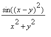> eps:=.5;

> plot3d(sin((x-y)^2)/(x^2+y^2),x=-eps..eps,y=-eps..eps,axes=framed);

The animation below shows the y= kx sections of this graph for various values of k.

To play the animation, click on the graph and then choose play from the animation menu.

Why does the animation tell you something about the above limit?

> animate(subs(y=k*x,sin((x-y)^2)/(x^2+y^2)),x=-eps..eps,k=-3..3);

Some Linear Approximations for a function F: -> .

Try changing the scale below - at least for the values scale =.1,.5 and 1.
(You need to re-execute the lines which follow after you change scale.)

The pictures compare the image of a certain square under the function F with

the image of the square under the linear approximation obtained at the center of

the square.
Compare the accuracy of linear approximation as a function of the size of the rectangle.

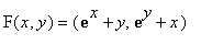Defining F: -> by . DF is its derivative at the point (x,y).

> F:=(x,y)->[1-exp(x)-y,1-exp(y)-x]; DF:=jacobian(F(x,y),[x,y]);

We will be linearizing F at the point p0. And scale controls the size of the rectangle we work with.

> scale:=1;
p0:=[.5*scale,.5*scale];

An easy way to draw a square with corner (0,0) and (scale,scale).

> gr1:=conformal(z,z=0..scale*(1+I)):
gr1a:=conformal(z,z=0..scale*(1+I),color=magenta):

This picture shows the original rectangle together with its image under F.

> F_gr:=transform(F):
display([gr1,F_gr(gr1)],title=`Image of Rectangle under F`);

Below is the corresponding picture under the linearization of F at p0.
Don't worry necessarily about the Maple code, but

F0= the image of the point p0 under F.
L=derivative DF at p0 (a 2 by 2 matrix)

L1=the linear approximation of F at p0

L2=a different form of L1 for Maple syntax reasons

> F0:=F(op(p0));
L:=map(evalf,subs({x=p0[1],y=p0[2]},eval(DF)));
L1:=convert(evalm(L &*vector([x-p0[1],y-p0[2]])+F0),list);
L2:=unapply(L1,[x,y]);
L2_gr:=transform(L2):
display([gr1a,L2_gr(gr1a)],title=`Image of Rectangle under Linear Approximation`);

Linearization at the Origin.

Try changing the scale below - at least for the values scale =.1,.5 and 1.

Why do the linearized pictures look the way they do?

Defining F: -> by . DF is its derivative at the point (x,y).

> F:=(x,y)->[1-exp(x)-y,1-exp(y)-x]; DF:=jacobian(F(x,y),[x,y]);

We will be linearizing F at the point p0. And scale controls the size of the rectangle we work with.

> scale:=0.1;
p0:=[0,0];

An easy way to draw a square with corner (0,0) and (scale,scale).

> gr1:=conformal(z,z=0..scale*(1+I)):
gr1a:=conformal(z,z=0..scale*(1+I),color=magenta):

This picture shows the original rectangle together with its image under F.

> F_gr:=transform(F):
display([gr1,F_gr(gr1)],title=`Image of Rectangle under F`);

Below is the corresponding picture under the linearization of F at p0.
Don't worry necessarily about the Maple code, but

F0= the image of the point p0 under F.
L=derivative DF at p0 (a 2 by 2 matrix)

L1=the linear approximation of F at p0

L2=a different form of L1 for Maple syntax reasons

> F0:=F(op(p0));
L:=map(evalf,subs({x=p0[1],y=p0[2]},eval(DF)));
L1:=convert(evalm(L &*vector([x-p0[1],y-p0[2]])+F0),list);
L2:=unapply(L1,[x,y]);
L2_gr:=transform(L2):
display([gr1a,L2_gr(gr1a)],title=`Image of Rectangle under Linear Approximation`);

Another function F: -> .

Try changing the scale below - at least for the values scale =1, .5, .1, .01.
(You need to re-execute the lines which follow after you change scale.)

The pictures compare the image of a certain square under the function F with

the image of the square under the linear approximation obtained at the center of

the square.
Compare the accuracy of linear approximation as a function of the size of the rectangle.

>

> F:=(x,y)->[x^2-y^2,2*x*y]; DF:=jacobian(F(x,y),[x,y]);

We will be linearizing F at the point p0. And scale controls the size of the rectangle we work with.

> scale:=1;
p0:=[.5*scale,.5*scale];

An easy way to draw a square with corner (0,0) and (-scale,-scale).

> gr1:=conformal(z,z=0..scale*(-1-I)):
gr1a:=conformal(z,z=0..scale*(-1-I),color=magenta):

This picture shows the original rectangle together with its image under F.

> F_gr:=transform(F):
display([gr1,F_gr(gr1)],title=`Image of Rectangle under F`);

Below is the corresponding picture under the linearization of F at p0.
Don't worry necessarily about the Maple code, but

F0= the image of the point p0 under F.
L=derivative DF at p0 (a 2 by 2 matrix)

L1=the linear approximation of F at p0

L2=a different form of L1 for Maple syntax reasons

> F0:=F(op(p0));
L:=map(evalf,subs({x=p0[1],y=p0[2]},eval(DF)));
L1:=convert(evalm(L &*vector([x-p0[1],y-p0[2]])+F0),list);
L2:=unapply(L1,[x,y]);
L2_gr:=transform(L2):
display([gr1a,L2_gr(gr1a)],title=`Image of Rectangle under Linear Approximation`);

>

Some Linear Approximations for a function F: -> .

The pictures compare the image of a certain square under the function F with

the image of the square under the linear approximation obtained at the center of

the square.

Try changing the scale below - at least for the values scale =2, 1, .5, .25, and .1.

Compare the accuracy of linear approximation as a function of the size of the rectangle.

> F:=(x,y)->[sin(x)*cos(y),sin(x)*sin(y),cos(x)]; DF:=jacobian(F(x,y),[x,y]);

We will be linearizing F at the point p0. And scale controls the size of the rectangle we work with.

> scale:=1;
p0:=[.5*scale,.5*scale];

An easy way to draw a square with corner (0,0) and (scale,scale).

> gr1:=conformal(z,z=0..scale*(1+I)):
gr1a:=conformal(z,z=0..scale*(+1+I),color=magenta):
display(gr1);

This picture shows the image under F.

The option scaling=constrained means to choose the same scale along all three axes.

> F_gr:=transform(F):
display(F_gr(gr1),title=`Image of Rectangle under F`,axes=framed,scaling=constrained);

Below is the picture of the image of the rectangle under the linearization of F at p0 together with the actual image.

Don't worry necessarily about the Maple code, but

F0= the image of the point p0 under F.
L=derivative DF at p0 (a 2 by 2 matrix)

L1=the linear approximation of F at p0

L2=a different form of L1 for Maple syntax reasons

> F0:=F(op(p0));
L:=map(evalf,subs({x=p0[1],y=p0[2]},eval(DF)));
L1:=convert(evalm(L &*vector([x-p0[1],y-p0[2]])+F0),list);
L2:=unapply(L1,[x,y]);
L2_gr:=transform(L2):
display([F_gr(gr1),L2_gr(gr1a)],title=`Image and its Linear Approximation`,axes=framed,scaling=constrained);

You could also try the above without the scaling=constrained option.

Can you explain what happens then?

>

>