![[Maple Plot]](quadthinkeval/quadric_think_eval1.gif)
Thinking Through Some Quadrics
Version .8
> with(plots):
Warning, the name changecoords has been redefined
Basic Paraboloid and Saddle
First look at the basic paraboloid vs. saddle dichotomy.:
Try rotating each (dragging with the left button on your mouse) to see how different each can look.
Note how much the second changes!
Can you see both algebraically and geometrically:
1. How the xz (i.e. y=0) and yz (i.e. x=0) sections compare
to each other
and in the two cases?
2. How the shape of the y=kx sections (for k a constant) vary in each example as a function of k?
3. Why the paraboloid graph has the 4 corners instead of being perfectly rounded?
4. What happens to these graphs as you change the coefficients of x and y but not their signs?
> plot3d(2*x^2+y^2,x=-1..1,y=-1..1,style=patchcontour,axes=normal,title=`paraboloid`);
> plot3d(x^2-y^2,x=-1..1,y=-1..1,style=patchcontour,axes=normal,title=`saddle`);
![[Maple Plot]](quadthinkeval/quadric_think_eval2.gif)
Seeing Roundness More Clearly
The view=-1..1 option just shows the portion of the graph where z is in this range and so
restores the expected circular symmetry to the paraboloid picture.
> plot3d(x^2+y^2,x=-1..1,y=-1..1,view=-1..1,style=patchcontour,axes=normal,title=`paraboloid with view option`);
![[Maple Plot]](quadthinkeval/quadric_think_eval3.gif)
Some Trickier Paraboloids and Saddles
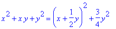
Algebraically each of these is of the form
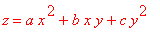 but geometrically they are
quite different.
1. Each is a paraboloid or saddle. Which is which?
2. Think about x=0 and y=0 sections. Can you tell them apart this way?
3. Think about y=x vertical sections. Does this distinguish?
4. What do horizontal z=constant sections look like for each?
5. Try thinking systematically about y=kx sections as a function of k to see if you can explain the pictures.
6. Completing the square can be used to systematically tell paraboloids form saddles. For example
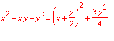 >= 0 always
> plot3d(x^2- x*y+ y^2,x=-1..1,y=-1..1,style=patchcontour,axes=normal,title=`figure 4`);
> plot3d(x^2+ 3*x*y+y^2,x=-1..1,y=-1..1,style=patchcontour,axes=normal,title=`figure 5`);
> plot3d(x^2+6*x*y+y^2,x=-1..1,y=-1..1,style=patchcontour,axes=normal,title=`figure 6`);
![]()
![[Maple Plot]](quadthinkeval/quadric_think_eval8.gif)
![[Maple Plot]](quadthinkeval/quadric_think_eval9.gif)
![[Maple Plot]](quadthinkeval/quadric_think_eval10.gif)
A Borderline Case
Each of these are parabolic cylinders.
1. Can you see why their shapes are so similar?
2. How do the two examples differ?
> plot3d(x^2,x=-1..1,y=-1..1,style=patchcontour,axes=normal,title=`figure 7`);
![[Maple Plot]](quadthinkeval/quadric_think_eval11.gif)
> plot3d(x^2- 2*x*y+ y^2,x=-1..1,y=-1..1,style=patchcontour,axes=normal,title=`figure 8`);
![[Maple Plot]](quadthinkeval/quadric_think_eval12.gif)
Hyperboloids
Can you see the relationship of the hyperboloid to the hyperbola?
> implicitplot3d(x^2+y^2-z^2=1,x=-2..2,y=-2..2,z=-2..2,axes=normal,title=`Hyperboloid 1`);
> implicitplot(x^2-z^2=1,x=-2..2,z=-2..2,title=`hyperbola`);
![[Maple Plot]](quadthinkeval/quadric_think_eval13.gif)
![[Maple Plot]](quadthinkeval/quadric_think_eval14.gif)
How about these two?
They are also closely related to the hyperbola above.
Do you see how?
> implicitplot3d(x^2+y^2-z^2=-1,x=-2..2,y=-2..2,z=-2..2,axes=normal,title=`Hyperboloid 2`);
> implicitplot3d(x^2+y^2-z^2=0,x=-2..2,y=-2..2,z=-2..2,axes=normal,title=`A Cone (missing a little bit)`);
![[Maple Plot]](quadthinkeval/quadric_think_eval15.gif)
![[Maple Plot]](quadthinkeval/quadric_think_eval16.gif)
The cone can be filled in more completely using the grid option
> implicitplot3d(x^2+y^2-z^2=0,x=-2..2,y=-2..2,z=-2..2,grid=[30,30,30],axes=normal,title=`A Cone More Completely`);
![[Maple Plot]](quadthinkeval/quadric_think_eval17.gif)
More to Think About
Some other things to try include :
1. What happens when you start adding terms linear in x, y, and z?
2. What will a general quadric usually look like?
3. What possibilities have we missed?
>
>
>
>