2D Plotting

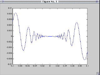
Plotting y=f(x) on the interval [-.1,.1]:

First create a vector of (e.g.) 200 equally spaces values between -.1 and .1.

x1=linspace(-.1,.1,200);

Suppose f(x) is an algebraic expression of standard functions such as f(x)= x^2*sin(1/x).

Then the following computes the y values from the x values.

y1 = x1 .^ 2 .* sin(1 ./ x1);

Now put up the plot:

plot(x1,y1)

Styles and colors mady be indicated e.g. by

plot(x,y,'r--')

where r indicates red, -- indicates dashed, : indicates dotted, and * means starred.

Titles, xlabels, ylabels, and text can be added by

title('Graph Illustrating ...') ; xlabel(' ... ') ; text(x0,y0,'string') etc.

Axes can be drawn by

axis([xmin xmax ymin ymax])

Adding Additional Graphs:

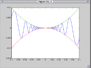
x2=linspace(-.1,.1,50);

(Note that this function oscillates less, so we take a coarser grid with only 50 points.

y2 = x2 .^2

y3 = -x2 .^2

plot(x1,y1,x2,y2,x2,y3)

Another Way to Combine Pictures:

Hold on

to cause additional pictures to be superimposed on the existing one

Hold off

to restore the default of replacing an old picture by a new one.

Plotting a Function Defined in an m-file:

[Mathlab Home | Math]