Analyzing the Population Changes

The state data for 1980 in the table of regional population distribution above could be entered in Maple using the commands:

with(linalg);
S[80] := vector( [.2167,.2599, .1906, .3327 ] );

You can enter the data S[90] for 1990 similarly.

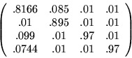
Let T be the 4 x 4 matrix

$$\left( \begin{array}{cccc} .8166 & .085 & .01 & .01 \\ .01 ... ...01 & .97 & .01 \\ .0744 & .01 & .01 & .97 \end{array} \right)$$

This problem will start out by testing the appropriateness of T as a possible transition matrix describing regional population shifts over a decade.

1.

By multiplying T on the left by the row vector [1,1,1,1], show that the sums of the columns of T are close to 1. (Explain why multiplying by this row vector is calculating the column sum.)

2.

Show that T approximately accounts for the change from 1980 to 1990, i.e. $T \circ S[80]$ is approximately S[90].

3.

Compute $T^{50} \circ S[80]$, $T^{100} \circ S[80]$, and $T^{200} \circ S[80]$, and compare these results. What does the comparison suggest ?

4.

Use the row operations package to approximately solve the system $T \circ w = w$. Explain why a state vector w satisfying this equation would represent an unchanging (steady-state ) population distribution for this model.
Maple Comments:

• Samples using the row operations package are located in the file :Maple V Release 4:Math 221: Row Operations Examples on each Macintosh in the Lab.
• To solve this system, you need only solve $A \circ w = 0$ where A is the matrix T-Id. The Maple commands

  Id := diag(1,1,1,1);
  A := T - Id;

  will generate these matrices.
• A single use of the row operations package to solve $A\circ x=b$ will include a read statement to load the package, a definition of A and b, a ``start_ge(A,b);'' call, and then a sequence of row operations (ar, mr and sr) as well as a back-substitution (bs()). For decimals, one can use (rounded_bs(k)) to round to k decimal places, thereby rounding small entries (from roundoff error) to zero.
• Note also, that in using the row operations package, you don't have to do arithmetic -- you can issue commands like:

  ar(1,2, .7865/.2345);

• By approximately solve, we mean just work to 4 digit accuracy in your row operations, and assume that naturally arising terms near 0 differ from 0 only because of roundoff error.
• There is a mathematically delicate issue associated with rounding here. The square system (T - Id)w=0 is solvable nontrivially only if T-Id is a singular matrix. Doing row operations with floating point may change this into a matrix that is non-singular although ``almost'' singular. A rigorous theory of when and how to replace an almost singular matrix by a singular one is somewhat difficult. Here we encourage you to just informally assume nearly zero entries are really zero. But this will only work if you do not unnaturally scale the entries. For example if you have a row every entry of which is 0 except for 0.00001, then rounding to 4 decimal places will round all entries to 0. But multiplying the row by 10⁵ to make this nonzero entry 1 would defeat the purpose of rounding.

5.

Compare your steady state answer to the result of $T^{100} \circ S[80]$ above. In converting your solution to one the sum of whose components is 1, you may find it helpful to use the Maple commands

v_sum := add(v[i],i=1..4);

if v is a vector or

v_sum := add(v[i,1],i=1..4);

if v is a 4 x 1 matrix to add up the 4 components of v and

mult := u -> u/v_sum;
map(mult,v);

The latter define a helper function multiplying any number by 1/v_sum, and then apply that function to each entry of v.

The transition matrix T is just one Markov chain model consistent with the data. You might find it interesting to think about other possibilities.

The fact that 3 and 4 agree can be shown to hold in general for Markov matrices as long as some power has all its entries strictly positive. But it's not obvious ....