Let
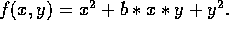 Using Maple, for
  and
and  ,
plot the gradients of f for
b=1, 2, and 4. Print these out. On each of these printouts, draw in by hand
(roughly) several level curves.
,
plot the gradients of f for
b=1, 2, and 4. Print these out. On each of these printouts, draw in by hand
(roughly) several level curves.
Problem 1
Let Using Maple, for
and ,
plot the gradients of f for
b=1, 2, and 4. Print these out. On each of these printouts, draw in by hand
(roughly) several level curves.
Problem 2
We can consider the derivative Df of a function f at a point  as
an approximation of f
by an affine linear function. (The word affine here refers to the fact that
these approximations have constant terms in them.) Here we explore this
linear approximation
aspect of the derivative.
as
an approximation of f
by an affine linear function. (The word affine here refers to the fact that
these approximations have constant terms in them.) Here we explore this
linear approximation
aspect of the derivative.
Consider the function

The corresponding first order approximation to f at the point  is
given by
is
given by

where 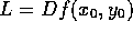 is the derivative of f at the point
Let C be a square of side  centered at the point
  , i.e.

For  taking on each ofthe values
  and
and  , do the
following:
, do the
following:
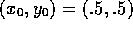 .
.
For each value of  , how do the images of C compare ?
What appears to be hapening as
, how do the images of C compare ?
What appears to be hapening as  decreases?
The Maple procedure transform_rect available in the Math 222 folders will be useful here. The output of transform_rect is a Maple graphics structure, so you can assign the result to a variable and then display several of these simultaneously.